
How to Build Machine Learning Model in Python in 2024
How to Build Machine Learning Model in Python in 2024
Did you know Python is the most popular language for machine learning – 57% of data scientists and machine learning developers use Python? No wonder it is, considering Python’s simplicity and powerful libraries, hence equally perfect for both the beginner and expert. Ready to dive into the world of machine learning? You’re at the right place!
I remember when I first started learning about machine learning, it seemed that every time I opened the book, I was staring at a mountain of heavy algorithms combined with mathematical equations. But let me tell you, once you break it down step by step, it is not as scary as it seems. As a matter of fact, it is just downright exciting.
Herein, we are going to describe how one can implement their very first machine learning model in Python. From setup, training, and evaluation of the model, this tutorial will take you through step by step. By the end of the article, you will feel confident and ready to get going with machine learning projects.
Now, go get your favorite drink, fire up your Python IDE, and let’s dive in!
Setting Up Your Python Environment for Machine Learning
Great, guys! Before we start exploring this exciting world of machine learning, we need to do some setup. You know, like in a kitchen when you want to prepare a really cool meal-you want all the ingredients ready and all your tools prepared and laid out!
First of all, let’s get the installation of Python on your machine. If you haven’t already, point your browser at python.org and download the latest version. I remember the first time I installed Python – excitedly, I practically did a happy dance the moment that “Hello, World!” printed out in the console.
Once you have Python up and running, there are some pretty important libraries you will want to add. These are the secret ingredients that will make your recipe for machine learning really shine:
- NumPy: This forms the basis of scientific computing in Python. If you use the analogy of flour in your pantry, you’re going to use it in almost everything!
- Pandas: This is like a Swiss Army knife if you deal with data manipulation and analysis.
- Scikit-learn: Scikit-learn is the Swiss Army knife of machine learning in Python. That library has multitudes of algorithms along with tools to make your life easy.
To install these libraries, fire up your command prompt or terminal and type:
pip install numpy pandas scikit-learn
Now, a pro tip I wished someone had told me when I started: use virtual environments! These are like different cooking stations for each of your projects. This way, you can have different versions of libraries for each project and not having other projects affect them. To create a virtual environment, use:
python -m venv myenv
And to activate it:
source myenv/bin/activate # On Unix or MacOS
myenv\Scripts\activate.bat # On Windows

Finally, here’s the import of those libraries in your Python script:
import numpy as np
import pandas as pd
from sklearn import model_selection, linear_model, metrics
That might seem like a lot but believe me, it’ll save you headaches down the line. Now we have our kitchen. err, our Python environment set up, ready to start cooking up some machine learning magic!
You will get into hiccups, so don’t stress when anything goes out of place in this step; been there, done that. Take a deep breath, Google the error message (a developer’s best friend), and keep trucking. You got this!
Understanding the Machine Learning Workflow
Now that we have our environment set up in Python, let’s talk about the machine learning workflow. Consider this your recipe for success-a way to get to your desired outcome, a series of steps that will yield a mouth-watering model of machine learning.
1. Data Collection and Preparation:
Really, this is where it all starts. You can’t bake a cake without ingredients, just like you can’t build any model of machine learning without data. I still remember my very first data collection project-scraping websites for hours after which I found that there was an API available. Do not be me, always search if somebody doesn’t have the dataset or API already!
Once you have your data, then you must clean it. This implies taking care of missing values and outliers, and making sure everything is in the right format. That’s essentially going through your groceries and checking no eggs are cracked.
2. Feature Selection and Engineering:
Well, features are the individual measurable properties of your data. Now, feature selection is a bit of an art-just like adding spices to your dish: if you add too few, the model will be flat and lack accuracy. Too many, and you mask the important signals with noise.
Feature engineering is where things can really get creative-maybe in combining existing features to create new ones, or transforming them in ways to better represent the underlying patterns. I remember spending days engineering features on a project, only to realize that all I needed was a simple logarithmic transformation of one variable. Sometimes less is more!
3. Model Selection:
It’s like choosing the right cooking method: will it be simple linear regression-the microwave dinner of machine learning, so to say-or complex neural networks, the sous-vide of algorithms? It all depends on your data, your problem, and your constraints.
4. Training and Testing:
Here’s where the magic happens: you split your data into training and testing sets, then turn your algorithm of choice loose on the training data. It’s a little like teaching a new chef your secret recipe-you show them how it’s done, then step back and see if they can replicate it.
5. Evaluation and Iteration:
Finally, you test your model on data it has not seen. How does it perform? Are its predictions correct? Here comes the accuracy and other metrics like precision and recall. If it is not perfect the first time around, don’t be discouraged. That’s the way machine learning works: iteration after iteration. Now, refine the features, adjust your algorithm, and try to run the model once again.
Remember, this workflow is not a one-way street. You will often find your-self looping back to earlier steps as you refine your model. This is like tasting your dish as you cook-in other words, you are constantly adjusting and improving.
Initially, I wished to rush through the steps for the preparation of data and engineering features, so that I might get to the “fun” part of training the model. Big mistake! I have come to realize very fast that quality in data and features can make or break your model. Nowadays, I am very easily prepared to invest up to 80% of my time in these critical early steps.
Each of these steps will be elaborated upon as we continue with the details in this tutorial. So for now, keep the above workflow in mind-it shall be your guide in the interesting domain of machine learning. Now, let’s get our hands dirty and start with the prepping of the dataset!
Preparing Your Dataset
All right, lovers of data! Time to roll up the sleeve and get our hands dirty with actual data. This step is not optional-the phrase “garbage in, garbage out” wasn’t coined for nothing. No matter how fancy your machine learning algorithm may be, it is going to fail if your data is a mess.
Well, first things first, let’s load our data in with Pandas. For the purpose of this example, let’s pretend we have a house prices dataset. Here’s how we might load it:
import pandas as pd
# Load the dataset
df = pd.read_csv(‘house_prices.csv’)
# Take a peek at the first few rows
print(df.head())
Each time I began, after an hour or two, I was deep in model building with little or no understanding of my data. Big mistake! Always take some time to understand your dataset. The following is a quick start to some basic EDA:
# Get basic information about the dataset
print(df.info())
# Check for missing values
print(df.isnull().sum())
# Get statistical summary of numerical columns
print(df.describe())
# For categorical columns, check unique values
for column in df.select_dtypes(include=[‘object’]).columns:
print(f”\nUnique values in {column}:”)
print(df[column].value_counts())
- Missing Values
Missing values will definitely sabotage your machine learning gears. Here’s a simple way to handle them:
# Fill numerical missing values with median
for column in df.select_dtypes(include=[‘float64’, ‘int64’]).columns:
df[column].fillna(df[column].median(), inplace=True)
# Fill categorical missing values with mode
for column in df.select_dtypes(include=[‘object’]).columns:
df[column].fillna(df[column].mode()[0], inplace=True)
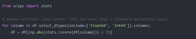
- Handling Outliers:
Outliers can bias your model’s performance. Here is a simple way to remove extreme outliers:
from scipy import stats
# Remove outliers (data points that are more than 3 standard deviations away)
for column in df.select_dtypes(include=[‘float64’, ‘int64’]).columns:
df = df[(np.abs(stats.zscore(df[column])) < 3)]
- Feature Scaling:
Most of the machine learning algorithms work better if the features are on a similar scale. Here is how you normalize your numerical features:
from sklearn.preprocessing import StandardScaler
scaler = StandardScaler()
numerical_columns = df.select_dtypes(include=[‘float64’, ‘int64’]).columns
df[numerical_columns] = scaler.fit_transform(df[numerical_columns])
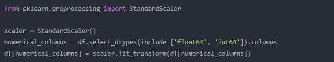
I still remember the first time I applied feature scaling – my model’s performance improved leaps and bounds! I had found my holy grail.
One last tip: do not forget to scale your categorical variables, too! Most algorithms cannot handle categorical data on their own. You have to encode them. The easiest way can be something like this using one-hot encoding; here is how you can do that in python:
df = pd.get_dummies(df, columns=df.select_dtypes(include=[‘object’]).columns)
That’s a lot, right? But believe me, this step in preparation is really one of the most important. I once struggled for weeks to try and improve a model’s performance, and literally my poor data preparation was what was causing the problem. Learn from my mistakes!
Remember, each dataset is different, and some techniques will need to be used over others in an attempt to work with your data. The important thing is to really understand your data so that when you start building models, you know exactly what you are doing. It is like a chef who tastes and readjusts his ingredients before he starts cooking or it sets the basic premise for all the subsequent work.
At last, we have clean data, scaled and ready to go; hence, we are one step closer to our aim of building a machine learning model. Exciting times ahead! We move on with the selection of the appropriate algorithm for our task.
Choosing the Right Machine Learning Algorithm
Well, members, our data is cleaned, features prepared, the moment of truth-high time for our selection of a machine learning algorithm. Now things can get really exciting!
The choice of algorithm is a choice of the right tool for the job. Wouldn’t someone use a sledgehammer when trying to hang a picture frame? Same principle here. Let’s describe some common algorithms and also the situations in which one might choose them.
- Linear Regression:
This is the most basic algorithm. It’s great for predicting a continuous value. If you’re trying to predict house prices based on square footage, this might be your go-to.
from sklearn.linear_model import LinearRegression
model = LinearRegression()

- Logistic Regression:
This is, despite the name suggesting otherwise, used in classification problems. It’s fantastic for binary outcomes, such as whether an email is spam or not.
from sklearn.linear_model import LogisticRegression
model = LogisticRegression()

- Decision Trees:
These are versatile, relatively simple to understand, and can be applied to classification and regression problems. Additionally, they support both numerical and categorical data as input.
from sklearn.tree import DecisionTreeClassifier
model = DecisionTreeClassifier()

I remember the first time I envisioned a decision tree. The algorithm’s train of thought just appeared before my eyes!
- Random Forest:
This is a collection of decision trees. Stronger than a single tree and less overfitting. To be used for complicated datasets.
from sklearn.ensemble import RandomForestClassifier
model = RandomForestClassifier()

- Support Vector Machines
These are powerful for both classification and regression, especially when the number of features is larger than the number of samples.
from sklearn.svm import SVC
model = SVC()

OK, now which one to decide upon? Well, here are some considerations:
- The nature of your problem at hand is a classification or regression problem.
- Size and quality of your dataset
- The number of features
- Interpretability requirements: some algorithms are more of a “black box” than others
- Computational resources available
Pro tip: don’t be afraid to try out a ton of different algorithms! I frequently have a workflow of starting with a super basic model (like linear regression) as a baseline then iteratively trying more advanced models in order to see if they provide better performance.
Scikit-learn makes trying a bunch of different algorithms super easy because of its standard API. Most models have the following form in python:
# Initialize the model
model = SomeModel()
# Fit the model to your training data
model.fit(X_train, y_train)
# Make predictions on new data
predictions = model.predict(X_test)
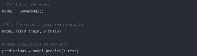
The above consistency makes it very easy to try out different algorithms without much modification in your code.
You’re basically getting a universal adapter for all your machine learning tools!
I remember starting out, spending hours in analysis paralysis over which algorithm to decide on. That’s changed now; it’s usually just better to start simple and iterate. Perfect should not be the enemy of good-you can always refine your choice later.
Another final consideration is something called the No Free Lunch Theorem. Concretely spoken, it says there is no single best algorithm that solves all problems best. What works on one dataset may be rather poor for another. Again, this underlines how important experimentation and options evaluation is.
Having discussed a few of the common algorithms and how to choose them, now it’s time to get our hands dirty with building our first machine learning model using linear regression!
Build Machine Learning Model in Python – Linear Regression
Alright, it’s showtime! We’re going to build our first machine learning model using linear regression. Why linear regression? It’s simple, interpretable, and it’s a great starting point for lots of problems. And it’s like the “Hello World” of machine learning – a rite of passage for every aspiring data scientist!
Lets say we are working with our house prices dataset, and we would like to predict the prices using square footage. Here is how we might do it:
- Splitting the Dataset
The first thing we want to do is split our data into our feature set (X) and our target variable set (y) and then into training and testing sets:
from sklearn.model_selection import train_test_split
# Assume ‘df’ is our DataFrame, ‘SqFt’ is our feature, and ‘Price’ is our target
X = df[[‘SqFt’]]
y = df[‘Price’]
X_train, X_test, y_train, y_test = train_test_split(X, y, test_size=0.2, random_state=42)
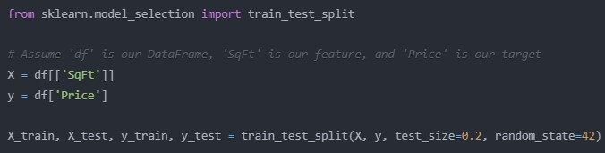
The test_size=0.2 means we’re using 80% of our data for training and 20% for testing. The random_state is just to ensure reproducibility.
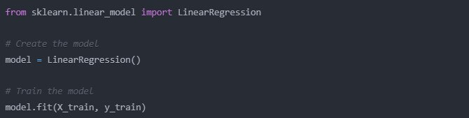
- Creating and training the model:
Now, let’s create our linear regression model and train it on our data:
from sklearn.linear_model import LinearRegression
# Create the model
model = LinearRegression()
# Train the model
model.fit(X_train, y_train)
That’s it! With these few lines of code, we have officially trained our very first machine learning model. It almost feels too easy, doesn’t it? But trust me, a lot is going on under the hood.
- Making predictions:
Finally, let’s use our model to make some predictions:
# Make predictions on the test set
y_pred = model.predict(X_test)

- Evaluating model performance:
Finally, let’s see how well our model is doing:
from sklearn.metrics import mean_squared_error, r2_score
# Calculate the Mean Squared Error
mse = mean_squared_error(y_test, y_pred)
print(f”Mean squared error: {mse}”)
# Calculate the R-squared score
r2 = r2_score(y_test, y_pred)
print(f”R-squared score: {r2}”)
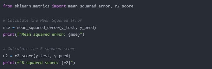
The Mean Squared Error gives us the average of the squared differences of our predictions and the actual values. Lower is better. The R-squared score gives us the proportion of the variance in the dependent variable predictable by the independent variable(s). It goes from 0 to 1 where 1 is a perfect fit.
I remember the first time I ran these metrics on a model that I’d built. The numbers stared back at me from the screen and for a second, I had no idea if they were good or bad. If you feel this way don’t worry – interpreting these metrics gets much easier with practice!
Here’s a cool trick: we can visualize our model’s predictions vs. the actual values:
import matplotlib.pyplot as plt
plt.scatter(X_test, y_test, color=’black’)
plt.plot(X_test, y_pred, color=’blue’, linewidth=3)
plt.xlabel(‘Square Footage’)
plt.ylabel(‘Price’)
plt.title(‘Linear Regression: Price vs Square Footage’)
plt.show()
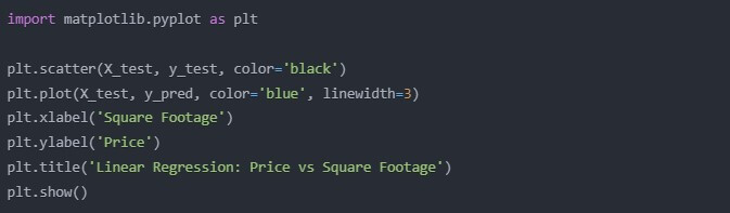
This will give you a nice visual representation of how well your model is doing. If the blue line-your model’s predictions-follows closely the pattern of the black dots-actual data points-you’re on the right track!
I know exactly what you’re thinking: “This is great, but how do I make it better?” Ah, my friend, that is where all the fun really begins. In the next section we will show how you can improve the performance of your model. But for now, take a moment and bask in the glory of your very first machine learning model. You have just taken a huge step into the world of AI – give yourself a pat on the back!
Improving Your Model’s Performance
Congratulations – you have built your first machine learning model! As any seasoned data scientist will tell you, however, your first model is rarely your best. In this section, let’s explore a few techniques to squeeze more performance out of our linear regression model.
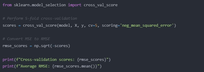
- Cross-validation:
You might recall we divided our data into training and testing sets. What if we just got unlucky and our test set wasn’t representative? Cross-validation is a way to guard against this by performing many train-test splits. How would we do that?
from sklearn.model_selection import cross_val_score
# Perform 5-fold cross-validation
scores = cross_val_score(model, X, y, cv=5, scoring=’neg_mean_squared_error’)
# Convert MSE to RMSE
rmse_scores = np.sqrt(-scores)
print(f”Cross-validation scores: {rmse_scores}”)
print(f”Average RMSE: {rmse_scores.mean()}”)
- Hyperparameter Tuning:
Many of the algorithms in machine learning are equipped with hyperparameters that can be optimised for better performance. In the context of linear regression, we don’t have that many hyperparameters to tune, but as an example, let’s consider Ridge regression – this is the regularised version of linear regression, where we penalise large intercepts and coefficients. Here is how this works in Python:
from sklearn.linear_model import Ridge
from sklearn.model_selection import GridSearchCV
# Define the parameter grid
param_grid = {‘alpha’: [0.1, 1, 10, 100]}
# Create a Ridge regression object
ridge = Ridge()
# Perform grid search
grid_search = GridSearchCV(ridge, param_grid, cv=5, scoring=’neg_mean_squared_error’)
grid_search.fit(X, y)
# Print the best parameters and score
print(f”Best parameters: {grid_search.best_params_}”)
print(f”Best RMSE: {np.sqrt(-grid_search.best_score_)}”)
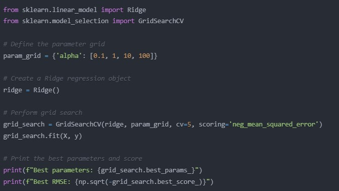
This is known as Grid Search where all the various combinations of parameters are tried out and the best is chosen. And so it is like having a tireless assistant who tries out all the various variants of the recipe to find the perfect one!
- Ensemble Methods:
Sometimes the wisdom of the crowd holds. Ensemble methods work by combining several models’ predictions. Let’s implement a simple ensemble between our linear regression model and a decision tree:
from sklearn.tree import DecisionTreeRegressor
from sklearn.ensemble import VotingRegressor
# Create the sub-models
model1 = LinearRegression()
model2 = DecisionTreeRegressor()
# Create the ensemble model
ensemble = VotingRegressor(estimators=[(‘lr’, model1), (‘dt’, model2)])
# Fit the ensemble model
ensemble.fit(X_train, y_train)
# Make predictions
ensemble_pred = ensemble.predict(X_test)
# Evaluate the ensemble model
ensemble_mse = mean_squared_error(y_test, ensemble_pred)
print(f”Ensemble MSE: {ensemble_mse}”)
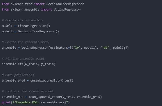
The first time I used an ensemble method, it felt like cheating-how could combining models be this effective? But it is a very valid and very powerful technique used by many top data scientists.
Remember, sometimes this might be an iterative process in model improvement: You may actually cycle between feature engineering, model selection, and these techniques to enhance performance. It’s like tuning a guitar: make small adjustments in the strings, test the sound, repeat until perfect.
One word of caution: watch out for overfitting. It is so tempting to try and squeeze out every last bit of performance on your training data. Always validate your improvements on a separate test set or using cross-validation.
I recall, early on, having spent hours at one point optimizing a model, only to find that it performed poorer on new, unseen data. It was humbling – it taught me an important lesson about finding that sweet spot between model complexity and generalization.
Enough of turbocharging our model – now onto one of my favorite parts: presenting or visualizing your results!
Visualizing Your Results
They say a picture is worth a thousand words, and in the world of machine learning, this couldn’t be truer. Visualizations can help you understand your data, interpret your model’s performance, and present your findings to others. Let’s find out ways of visualizing our results using Matplotlib and Seaborn.
- Residual Plot:
A residual plot will always help us to verify if our assumptions of linear regression are satisfied. It plots the residuals, differences between the predicted and actual values, against the predicted values:
import matplotlib.pyplot as plt
import seaborn as sns
# Calculate residuals
residuals = y_test – y_pred
# Create residual plot
plt.figure(figsize=(10, 6))
plt.scatter(y_pred, residuals)
plt.xlabel(‘Predicted Values’)
plt.ylabel(‘Residuals’)
plt.title(‘Residual Plot’)
plt.axhline(y=0, color=’r’, linestyle=’–‘)
plt.show()
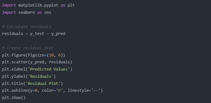
If you see a random scatter of points around the horizontal line at y=0, great! That suggests our linear regression assumptions are likely met. If you see patterns in this plot, it may indicate that the linear model is not an adequate fit for our data.
- Actual vs Predicted Plot:
This plot visualizes the how well predicted values match actual values:
plt.figure(figsize=(10, 6))
plt.scatter(y_test, y_pred)
plt.plot([y_test.min(), y_test.max()], [y_test.min(), y_test.max()], ‘r–‘, lw=2)
plt.xlabel(‘Actual Values’)
plt.ylabel(‘Predicted Values’)
plt.title(‘Actual vs Predicted’)
plt.show()

The closer the points are to the red dashed line, the better our predictions. I remember that when I first ever made this plot it was so satisfying to be able to see that points clustered around the line!
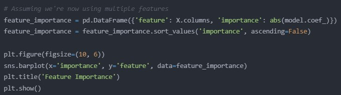
- Feature Importance (for multiple features):
If we are using multiple features then we may well want to know which ones are most important. Provided we are using linear regression then we can look at the absolute values of the coefficients:
# Assuming we’re now using multiple features
feature_importance = pd.DataFrame({‘feature’: X.columns, ‘importance’: abs(model.coef_)})
feature_importance = feature_importance.sort_values(‘importance’, ascending=False)
plt.figure(figsize=(10, 6))
sns.barplot(x=’importance’, y=’feature’, data=feature_importance)
plt.title(‘Feature Importance’)
plt.show()
- Correlation Heatmap:
If you have multiple features, a correlation heatmap can help you understand relationships between them:
plt.figure(figsize=(12, 10))
sns.heatmap(X.corr(), annot=True, cmap=’coolwarm’)
plt.title(‘Correlation Heatmap’)
plt.show()
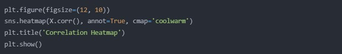
This plot is like a treasure map for feature selection. Highly correlated features might be redundant and one could remove some without losing much information.
- Distribution of Target Variable:
Understanding the distribution of your target variable can be very important:
plt.figure(figsize=(10, 6))
sns.histplot(y, kde=True)
plt.title(‘Distribution of Target Variable’)
plt.xlabel(‘Value’)
plt.ylabel(‘Frequency’)
plt.show()
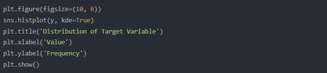
If your target variable is highly skewed, you may want to consider transforming it (e.g., using log transformation) to make it closer to normally distributed.
Keep in mind that these visualizations are not only for you, but they’re also great ways of presenting your findings to other people. I had this stakeholder once who was very skeptical regarding the value our machine learning project. So once I showed them these visualizations, he could see for himself-the patterns and insight. It was like watching a lightbulb turn on!
And by all means, play with different plot types and color schemes until your point comes across intuitively and as clear as possible. After all, why can’t data science be beautiful?
Having visually explored our results, let’s finish this off by talking about common pitfalls and how to avoid them.
Common Pitfalls and How to Avoid Them
As we get closer to the end of our journey into building machine learning models, it is necessary to touch base on some common pitfalls that even the most seasoned data scientists can be subjected to. Knowledge of these will make you better prepared for building robust and reliable models. So, let’s dive in!
1. Overfitting:
Ah, overfitting-the bane of many a data scientist’s existence. That’s like memorizing the answers to a test, not truly understanding the material. Your model is doing great on the training data but then fares abysmally at new, unseen data.
How to avoid it:
- Do cross-validation to get a more robust estimate of the performance of your model.
- Try simpler models or use regularization techniques-say, Lasso or Ridge regression.
- If possible, collect more data.
I once spent weeks fine-tuning a model to get near-perfect performance on my training data. I was thrilled! Until I tested it on new data and watched it fail spectacularly. Well, that was a humbling experience; it taught me the importance of generalization.
2. Underfitting:
The opposite of overfitting, underfitting is a situation where your model is too simple to model the underlying structure in your data.
How to avoid it:
- Try more complex models or ensemble methods.
- Feature engineering: create new features or transform the existing ones.
- In case of regularization, try lowering the regularization strength.
3. Not Handling Imbalanced Datasets:
This is important in classification problems. For instance, if 99% of your data belongs to one class, a model which constantly predicts that class will be 99% accurate-but utterly useless!
How to avoid it:
- Use appropriate evaluation metrics: instead of just using accuracy, use precision, recall, F1-score.
- Either oversample the minority class, or undersample the majority.
- Utilize algorithms which work with imbalanced data directly, such as decision trees, with adjusted class weights.
4. Feature Leakage
This occurs when your model is exposed during training to information that it wouldn’t have at the time of making a prediction in the real world. It’s like having the answers, sealed in the flap at the back of the exam book.
How to avoid it:
- Be careful with time-based data. Never use future information in order to predict the past.
- Wherever pre-processing the data is involved such as scaling or imputation of missing values, do it separately for both train and test.
- Be suspect of features seeming suspiciously good: They might be leaking information.
I once worked on a project where our model was performing suspiciously well. After some digging, we realized one of our features was essentially a proxy for the target variable. Removing it brought our performance back down to earth, but gave us a much more reliable and generalizable model.
5. Ignoring Domain Knowledge:
While machine learning can uncover patterns we might miss, it’s dangerous to ignore subject matter expertise.
How to avoid it:
- Always involve domain experts on your project.
6. Not Interpreting Your Model
Black-box models may perform well, but sometimes if you can’t explain how they work, that makes it hard to gain much insight or trust them.
How to avoid it:
- Start with the simple, more interpretable models when possible.
- Use techniques like SHAP values in order to interpret complex models.
- Always explain your model’s decisions in plain language.
Remember, the goal of machine learning isn’t just to make accurate predictions-it’s to gain insights and make better decisions. A model you can’t explain is like a car with a great engine but no steering wheel!
Let me end by reiterating that you learn from mistakes. The more pitfalls you fall into and climb out of, the better a data scientist you become. I have fallen into every one of these traps in my career so far and each time emerged wiser.
Conclusion
Wow, it’s been a ride! In this course, we spoke about a lot: from setting up your Python environment to creating and improving your first machine learning model. Now that we are coming toward the end, let’s revisit the major steps we’ve learned:
- We started by installing the Python environment: we installed essential libraries such as NumPy, Pandas, and Scikit-learn.
- Full immersion into the workflow of machine learning gave us an idea of how important each one of these steps is, from data collection to model evaluation.
- We were able to learn how to prepare our dataset, handle missing values, deal with outliers, and scale our features.
- We learned different algorithms for machine learning and how to select the right one based on the nature of our problem.
- We have completed our first machine learning model using linear regression: learning how to split our data, train our model, and then make predictions.
- We learned various methods to improve the performance of our model, such as crossvalidation, hyperparameter tuning and ensemble methods.
- We also visualized our results through a host of different plots for the purposes of communicating and understanding our findings.
- Finally, we discussed common pitfalls in machine learning and how to avoid those.
Remember that the construction of machine learning models is as much an art as it is science. It takes a good level of creativity, intuition, and a lot of practice. And do not be discouraged if your first models are not quite doing as well as you may have hoped-the best- every seasoned data scientist has been there!
As you continue in your journey in machine learning here are some final thoughts to keep in mind:
- Simple start: Use the simplest models first, adding complexity as required. One will be astonished at how often such simple models do a pretty decent job.
- Understand the data: Understand and have a feel for one’s data through summary statistics and visualization before modeling. The insights gained thereby might turn out to be priceless.
- Iterate: Machine learning is essentially an iterative process, and no one gets it right the first time. Through every iteration, go back, review, and refine your approach.
- Be curious: Machine learning is a rapidly evolving field; keep learning about the latest techniques and do not be afraid to try something new.
- Share and collaborate: Contribute to online forums or communities, participate in Kaggle competitions, or start working on some open-source project. You will find yourself learning much faster when learning with and from others.
- Ethics matter: As you get more proficient, never stop thinking about the models you make from an ethical point of view. Machine learning can greatly affect people’s lives, so use your powers for good.
I still remember the amazement that engulfed me the first time I actually managed to build a machine-learning model that worked. For a moment, I felt superhuman-unleashed, I could predict stuff and find patterns in data like never before. That thrill of excitement and possibility has remained within me all these years in the field.
Now it is your turn to try, learn, create. Do not be afraid to make mistakes; often, they are the best teachers. And always remember that every master started out an apprentice. With persistence and passion, you will be amazed what you can accomplish.
So, what are you waiting for? Fire up that Python environment, load up a dataset, and start building! The world of machine learning is at your fingertips, and who knows? Your next model might just change the world.
Happy modeling, and may your predictions be ever accurate!